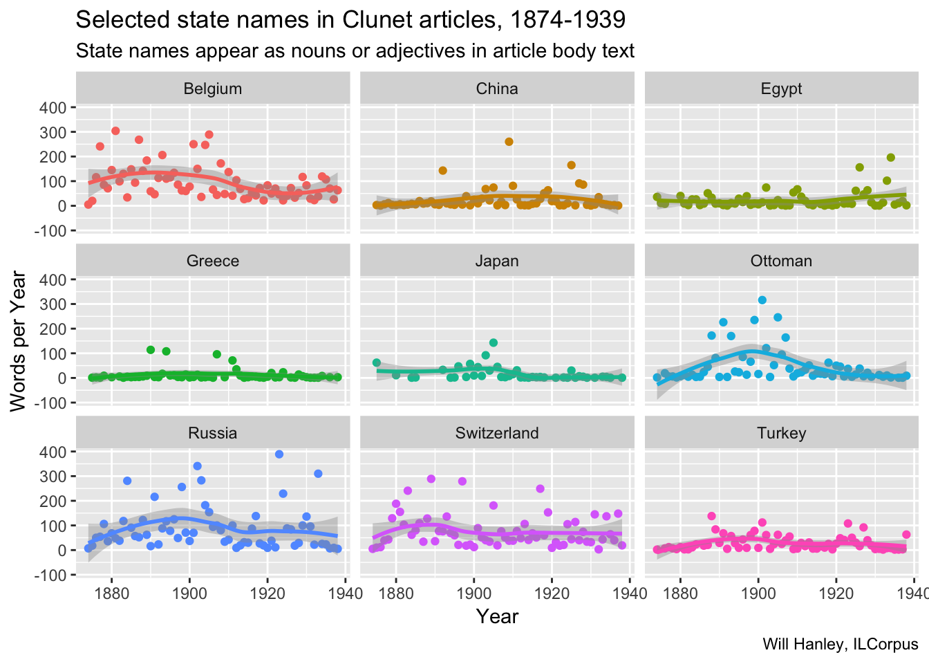
States in Clunet articles

Posted at — Jun 13, 2019

This chart counts references to selected states the standalone articles in Clunet. The pattern seems to differ from the pattern in jurisprudence. Egypt is less prominent, while the Ottomans and Russia are more prominent. China, Greece, and Japan show a few outlying points, most produced by a single article focused on that state.

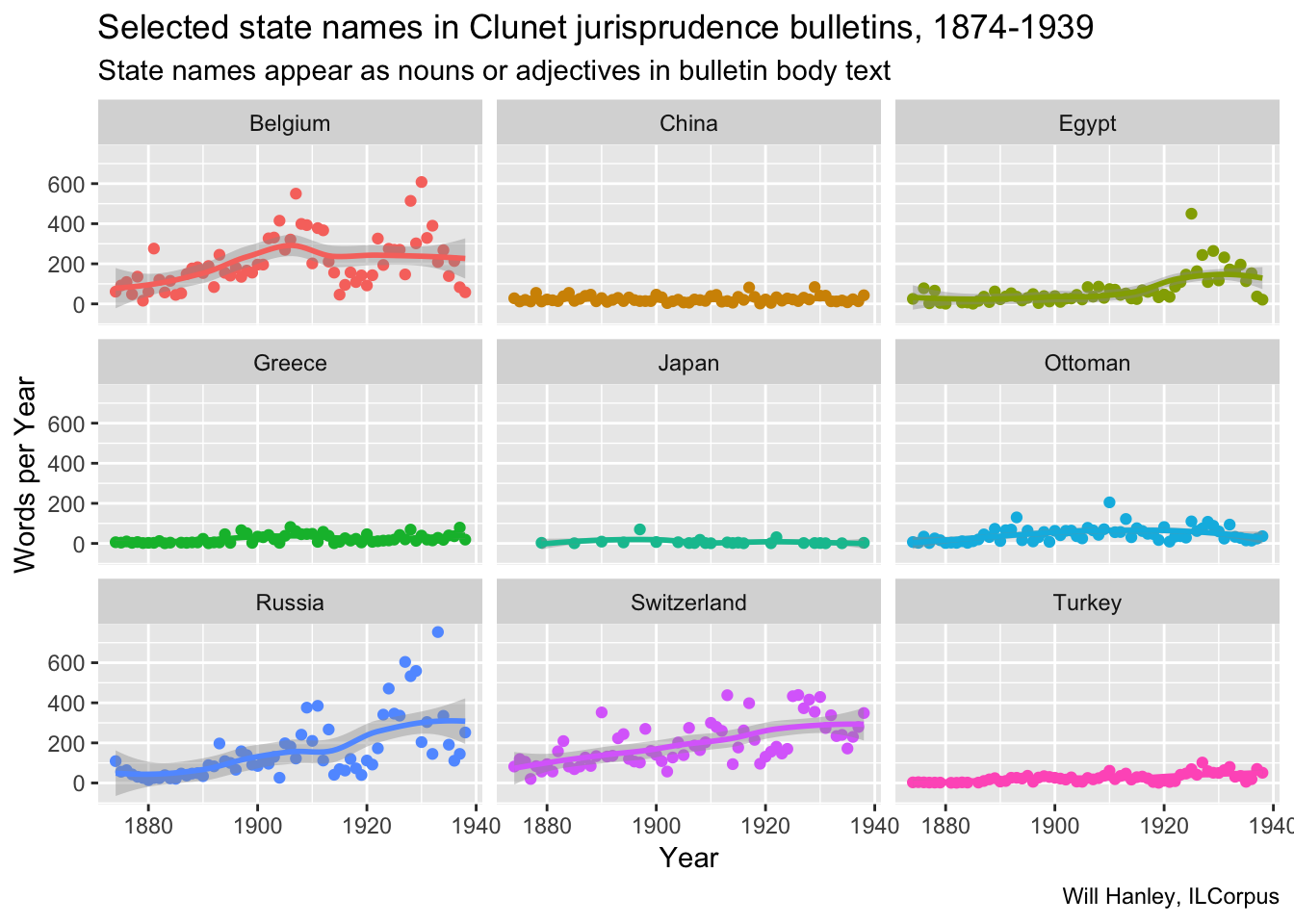
If we look at the pattern of occurence of the same words in the test of the jurisprudence bulletins themselves, we notice that the Ottoman empire and Turkey are less prominent. We also notice that here there are no spikes for China, Greece, and Japan.

Underlying code

library(xml2)
library(tidyverse)
library(tokenizers)
library(ggplot2)

#load folder of files
clunet_files <- dir("~/GitHub/ilcorpus/journals/clunet/clunet-issues", full.names = TRUE)

# this function extracts text and metadata
extract_data <- function(file){xml_find_all(xml_child(read_xml(file), 2), ".//d1:div") %>% 
    lapply(function(x) {
      list(
        type = xml_attr(x, "type"),
        feature = xml_attr(x, "feature"),
        text = xml_text(x)
      )
    }) %>% bind_rows()
}

# run on folder of files
clunet_words_list <- lapply(clunet_files, extract_data)

# unnest to make one big tibble
unnested_clunet_words <-tibble(index = 1:length(clunet_words_list), value = clunet_words_list) %>% unnest()

# fetch metadata to join table with dates
clunet_metadata <- read_csv("~/GitHub/ilcorpus/journals/clunet/clunet-summary.csv")
clunet_words <- clunet_metadata %>%
  inner_join(unnested_clunet_words)  %>%
  select(year, type, feature, text)

# articles only
clunet_article_words <- clunet_words %>%
  filter(type == "article") %>%
  mutate(words = tokenize_words(text)) %>% 
  select(-text) %>% 
  select(-feature) %>% 
  select(-type) %>% 
  unnest() 

# single count per year
unique_clunet_article_words <- clunet_article_words %>% 
  add_count(words, year, sort = TRUE) %>% 
  distinct()

# state by state breakdown
egypt <- unique_clunet_article_words %>% 
  filter(grepl(".gypt.+", words)) %>% 
  group_by(year) %>% 
  summarise(count = sum(n)) %>% 
  add_column(state = "Egypt")
belgium <- unique_clunet_article_words %>% 
  filter(grepl("belg.+", words)) %>% 
  group_by(year) %>% 
  summarise(count = sum(n)) %>% 
  add_column(state = "Belgium")
switzerland <- unique_clunet_article_words %>% 
  filter(grepl("suis.+", words)) %>% 
  group_by(year) %>% 
  summarise(count = sum(n)) %>% 
  add_column(state = "Switzerland")
china <- unique_clunet_article_words %>% 
  filter(grepl("chin.+", words)) %>% 
  group_by(year) %>% 
  summarise(count = sum(n)) %>% 
  add_column(state = "China")
japan <- unique_clunet_article_words %>% 
  filter(grepl("japon.+", words)) %>% 
  group_by(year) %>% 
  summarise(count = sum(n)) %>% 
  add_column(state = "Japan")
turkey <- unique_clunet_article_words %>% 
  filter(grepl("turq.+", words)) %>% 
  group_by(year) %>% 
  summarise(count = sum(n)) %>% 
  add_column(state = "Turkey")
greece <- unique_clunet_article_words %>% 
  filter(grepl("grec.*", words)) %>% 
  group_by(year) %>% 
  summarise(count = sum(n)) %>% 
  add_column(state = "Greece")
ottoman <- unique_clunet_article_words %>% 
  filter(grepl("otto.+", words)) %>% 
  group_by(year) %>% 
  summarise(count = sum(n)) %>% 
  add_column(state = "Ottoman")
russia <- unique_clunet_article_words %>% 
  filter(grepl("russ.+", words)) %>% 
  group_by(year) %>% 
  summarise(count = sum(n)) %>% 
  add_column(state = "Russia")
  
# make tibble
states_count <- full_join(belgium, switzerland)
states_count <- full_join(egypt, states_count)
states_count <- full_join(china, states_count)
states_count <- full_join(japan, states_count)
states_count <- full_join(turkey, states_count)
states_count <- full_join(greece, states_count)
states_count <- full_join(ottoman, states_count)
states_count <- full_join(russia, states_count)
states_count

# make plot
p <- ggplot(data = states_count, mapping = aes(x = year, y = count, color = state))
p + geom_point() + geom_smooth() + 
  facet_wrap(~state) +
  scale_y_continuous() +
  theme(legend.position="none") +
  labs(x = "Year", 
       title = "Selected state names in Clunet articles, 1874-1939", 
       subtitle = "State names appear as nouns or adjectives in article body text",
       y = "Words per Year",
       caption = "Will Hanley, ILCorpus")

# same thing for bulletins
clunet_bulletin_words <- clunet_words %>%
  filter(type == "bulletin") %>%
  mutate(words = tokenize_words(text)) %>% 
  select(-text) %>% 
  select(-feature) %>% 
  select(-type) %>% 
  unnest() 

# single count per year
unique_clunet_bulletin_words <- clunet_bulletin_words %>% 
  add_count(words, year, sort = TRUE) %>% 
  distinct()

# state by state breakdown
egypt_b <- unique_clunet_bulletin_words %>% 
  filter(grepl(".gypt.+", words)) %>% 
  group_by(year) %>% 
  summarise(count = sum(n)) %>% 
  add_column(state = "Egypt")
belgium_b <- unique_clunet_bulletin_words %>% 
  filter(grepl("belg.+", words)) %>% 
  group_by(year) %>% 
  summarise(count = sum(n)) %>% 
  add_column(state = "Belgium")
switzerland_b <- unique_clunet_bulletin_words %>% 
  filter(grepl("suis.+", words)) %>% 
  group_by(year) %>% 
  summarise(count = sum(n)) %>% 
  add_column(state = "Switzerland")
china_b <- unique_clunet_bulletin_words %>% 
  filter(grepl("chin.+", words)) %>% 
  group_by(year) %>% 
  summarise(count = sum(n)) %>% 
  add_column(state = "China")
japan_b <- unique_clunet_bulletin_words %>% 
  filter(grepl("japon.+", words)) %>% 
  group_by(year) %>% 
  summarise(count = sum(n)) %>% 
  add_column(state = "Japan")
turkey_b <- unique_clunet_bulletin_words %>% 
  filter(grepl("turq.+", words)) %>% 
  group_by(year) %>% 
  summarise(count = sum(n)) %>% 
  add_column(state = "Turkey")
greece_b <- unique_clunet_bulletin_words %>% 
  filter(grepl("grec.*", words)) %>% 
  group_by(year) %>% 
  summarise(count = sum(n)) %>% 
  add_column(state = "Greece")
ottoman_b <- unique_clunet_bulletin_words %>% 
  filter(grepl("otto.+", words)) %>% 
  group_by(year) %>% 
  summarise(count = sum(n)) %>% 
  add_column(state = "Ottoman")
russia_b <- unique_clunet_bulletin_words %>% 
  filter(grepl("russ.+", words)) %>% 
  group_by(year) %>% 
  summarise(count = sum(n)) %>% 
  add_column(state = "Russia")

# make tibble
states_count_b <- full_join(belgium_b, switzerland_b)
states_count_b <- full_join(egypt_b, states_count_b)
states_count_b <- full_join(china_b, states_count_b)
states_count_b <- full_join(japan_b, states_count_b)
states_count_b <- full_join(turkey_b, states_count_b)
states_count_b <- full_join(greece_b, states_count_b)
states_count_b <- full_join(ottoman_b, states_count_b)
states_count_b <- full_join(russia_b, states_count_b)
states_count_b

# make plot
p_b <- ggplot(data = states_count_b, mapping = aes(x = year, y = count, color = state))
p_b + geom_point() + geom_smooth() + 
  facet_wrap(~state) +
  scale_y_continuous() +
  theme(legend.position="none") +
  labs(x = "Year", 
       title = "Selected state names in Clunet jurisprudence bulletins, 1874-1939", 
       subtitle = "State names appear as nouns or adjectives in bulletin body text",
       y = "Words per Year",
       caption = "Will Hanley, ILCorpus")

International Law Corpus

Visualizations of international law periodical content, 1869-1939.

States in Clunet articles

Underlying code