Counting states in jurisprudence reports

Posted at — Jun 6, 2019

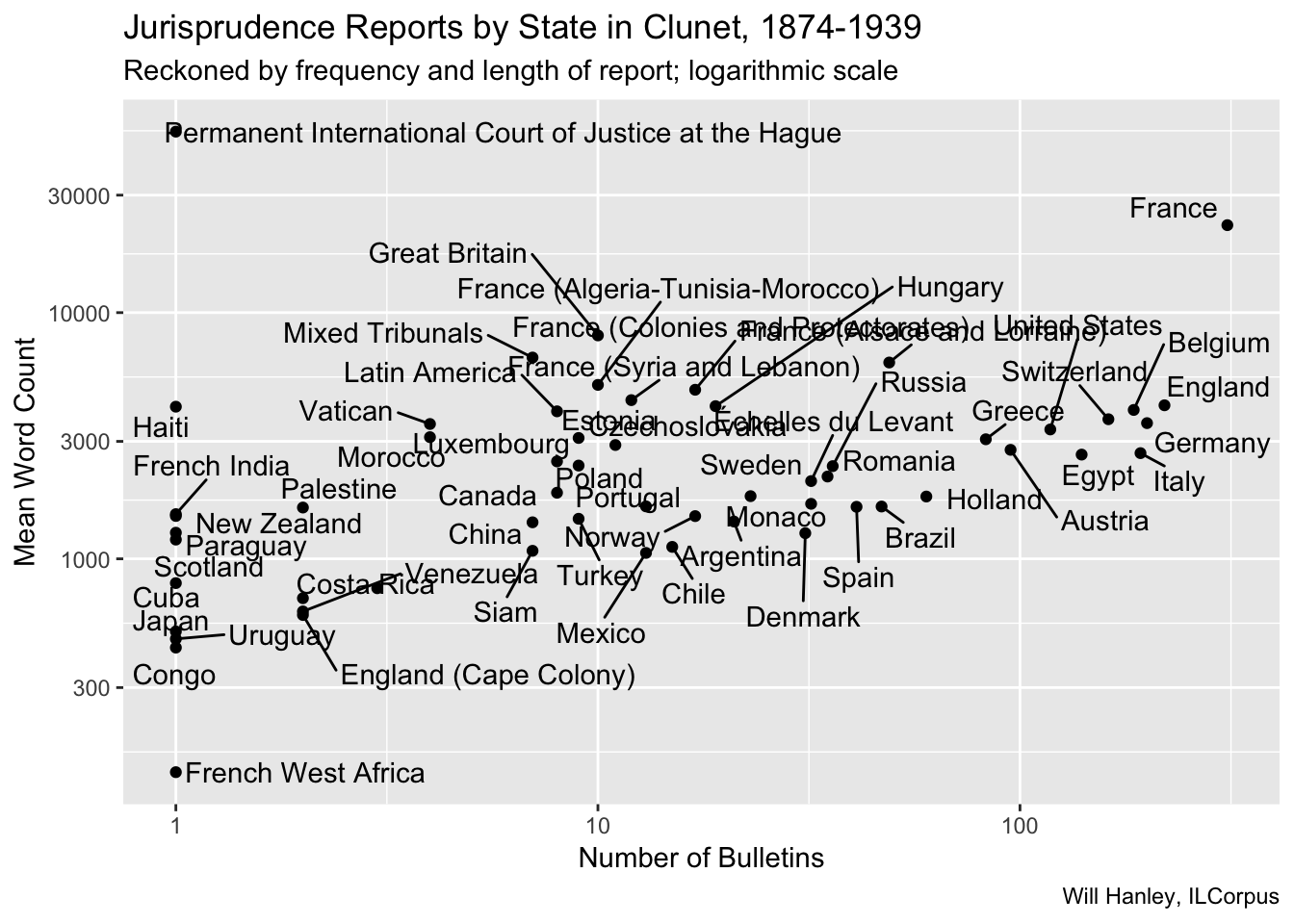
The “Jurisprudence” section of Clunet contains thousands of “bulletins” reporting decisions. The section is subdivided by state. This scatterplot captures the number of bulletins for each state and their average length.

Number of bulletins is one proxy for the notability of a state. Of course, not all of these states were present throughout the sixty-five year period. I’ll break out time series in future graphs.

Length of bulletin is one proxy for the depth of engagement with jurisprudence. At present this measure slightly misrepresents the jurisprudence bulletins, however. Many bulletins contained more than one report, but I have not yet managed to subdivide this section of the journal.

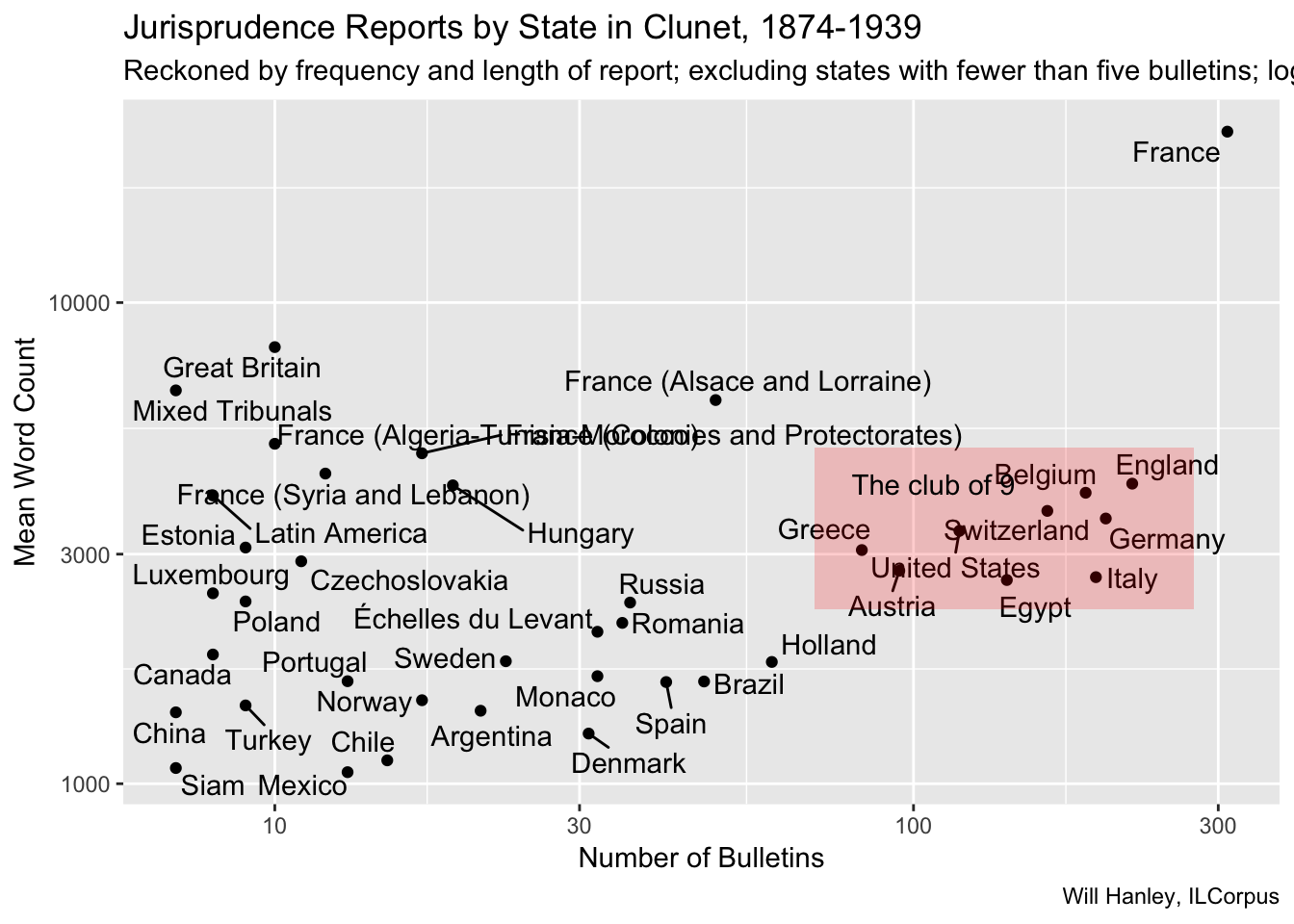
This plot shows only those states with more than five jurisprudence bulletins. Clearly France is an outlier both in terms of count and length. A relatively compact group of nine states comes next in prominence.

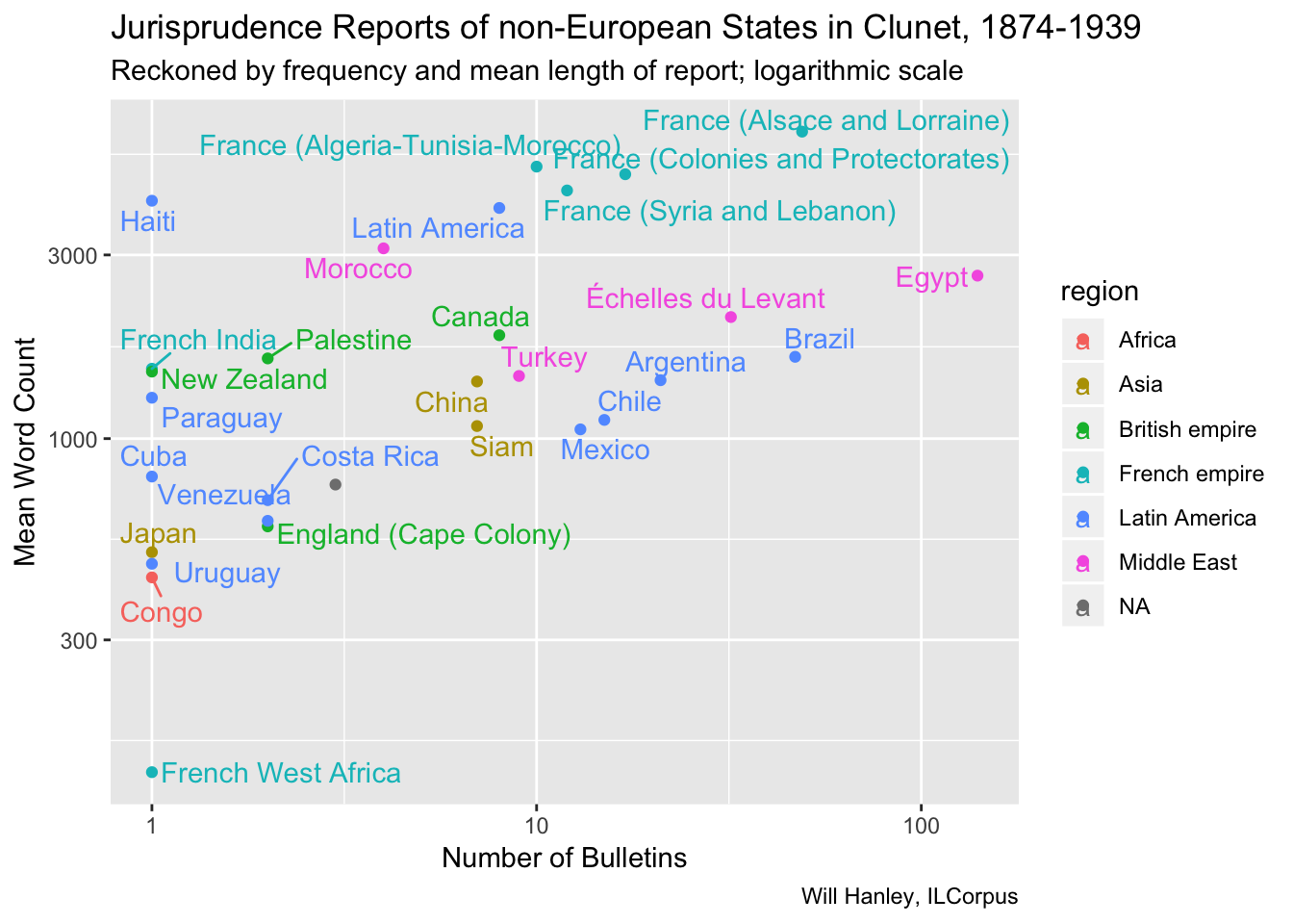
Among non-European states, Egypt is most prominent. Brazil and the “Échelles du Levant” (non-Ottoman Mediterranean ports subject to the capitulations) come next. A cluster of French colonies stands out, and Latin American states are relatively numerous. Asian states are remarkable for their slight presence.

Underlying code

library(tidyverse)
library(tokenizers)
library(ggplot2)
library(socviz)
library(ggrepel)

#load folder of files
clunet_files <- dir("~/GitHub/ilcorpus/journals/clunet/clunet-issues", full.names = TRUE)

# function to extract word count and metadata for divs within jurisprudence
extract_state_data <- function(x){
  # read file
  file <- read_xml(x)
  # extract divs
  divs <- file %>% xml_find_all(".//d1:div[@feature='jurisprudence']/d1:div")
  # get state attribute 
  state_code <- divs %>% xml_attr("state")
  filename <- x %>% gsub(".+/GitHub/ilcorpus/journals/[a-z]+/[a-z,-]+/", "", .) %>% gsub(".xml", "", .)
  year <- x %>% gsub(".+/GitHub/ilcorpus/journals/[a-z]+/[a-z,-]+/[a-z]+-", "", .) %>% gsub("-..xml", "", .)
  
  #find the head and word count for each div
  #returns a list of data frames
  output <- lapply(divs, function(d){
    header <- d %>% 
      xml_find_first(".//d1:head") %>% 
      xml_text() %>% 
      paste(collapse=" ") %>% 
      gsub("\\s+", " ", .)
    text <- d %>% 
      xml_find_all(".//d1:p") %>% 
      xml_text() %>% 
      paste(collapse=" ") %>% 
      gsub("\\s+", " ", .)
    count <- length(tokenize_words(text)[[1]])
    tibble(head=header, count)
  })
  #bind everything up into a tibble.
  answer <- do.call(rbind, output)
  test_tibble <- cbind(tibble(filename = filename, year = as.numeric(year), state_code = state_code), answer)
}

# run function and make tibble
clunet_states <- lapply(clunet_files, extract_state_data)
one_list <- do.call(rbind, clunet_states)
clunet_states_tibble <- as_tibble(one_list, .name_repair = "minimal")

# load state names file
state_names <- read_tsv("~/GitHub/ilcorpus/codes/state-codes.tsv")

# get mean word count and count of reports, join with state names
clunet_states_sum <- clunet_states_tibble %>% 
  group_by(state_code) %>% 
  summarise(words = mean(count), reports = n()) %>% 
  left_join(state_names)

# all-states scatterplot
p <- ggplot(data = clunet_states_sum, mapping = aes(x = reports, y = words, label = state))
p + geom_point() + 
  geom_text_repel() +
  scale_x_log10() +
  scale_y_log10() +
  labs(x = "Number of Bulletins", 
       title = "Jurisprudence Reports by State in Clunet, 1874-1939", 
       subtitle = "Reckoned by frequency and length of report; logarithmic scale", 
       y = "Mean Word Count",
       caption = "Will Hanley, ILCorpus")

# states with >5 count scatterplot
p1 <- ggplot(data = (subset(clunet_states_sum, reports > 5)), 
             mapping = aes(x = reports, y = words, label = state))
p1 + geom_point() + 
  geom_text_repel() +
  scale_x_log10() +
  scale_y_log10() +
  labs(x = "Number of Bulletins", 
       title = "Jurisprudence Reports by State in Clunet, 1874-1939", 
       subtitle = "Reckoned by frequency and length of report; excluding states with fewer than five bulletins; logarithmic scale", 
       y = "Mean Word Count",
       caption = "Will Hanley, ILCorpus") +
  annotate(geom = "rect", xmin = 70, xmax = 275, 
           ymin = 2300, ymax = 5000, fill = "red", alpha = 0.2) +
  annotate(geom = "text", x = 80, y = 4200, label = "The club of 9", hjust = 0)

# non-European state scatterplot
p2 <- ggplot(data = subset(clunet_states_sum, region %nin% c("Europe", "North America", "International", "NA")), mapping = aes(x = reports, y = words, label = state, color = region))
p2 + geom_point() + 
  geom_text_repel() +
  scale_x_log10() +
  scale_y_log10() +
  labs(x = "Number of Bulletins", 
       title = "Jurisprudence Reports of non-European States in Clunet, 1874-1939", 
       subtitle = "Reckoned by frequency and mean length of report; logarithmic scale", 
       y = "Mean Word Count",
       caption = "Will Hanley, ILCorpus")

International Law Corpus

Visualizations of international law periodical content, 1869-1939.

Counting states in jurisprudence reports

Underlying code