Journal word counts over time

Posted at — May 28, 2019

The sixty million words in the first version of the international law corpus are distributed over time like this:

This graph distinguishes between three journals: the Journal du droit international privé et de la jurisprudence comparée (“clunet”, in yellow), the Bulletin de la Société de législation comparée (“bslc”, in orange), and the Revue de droit international et de législation comparée (“rdilc”, in green).

It shows a steady rise in overall publishing volume until the 1890s. From the beginning of the 1890s to the end of the 1920s, the total word count of these three journals typically hovered around one million per year. The influence of World War One is marked: the RDILC stopped publication altogether, while Clunet produced its largest volume in 1917. After 1930, overall word volume wanes.

This chart, which does not show a combined word count for the three journals, shows that the rise and fall in Clunet’s volume is largely responsible for the overall shape of the first graph.

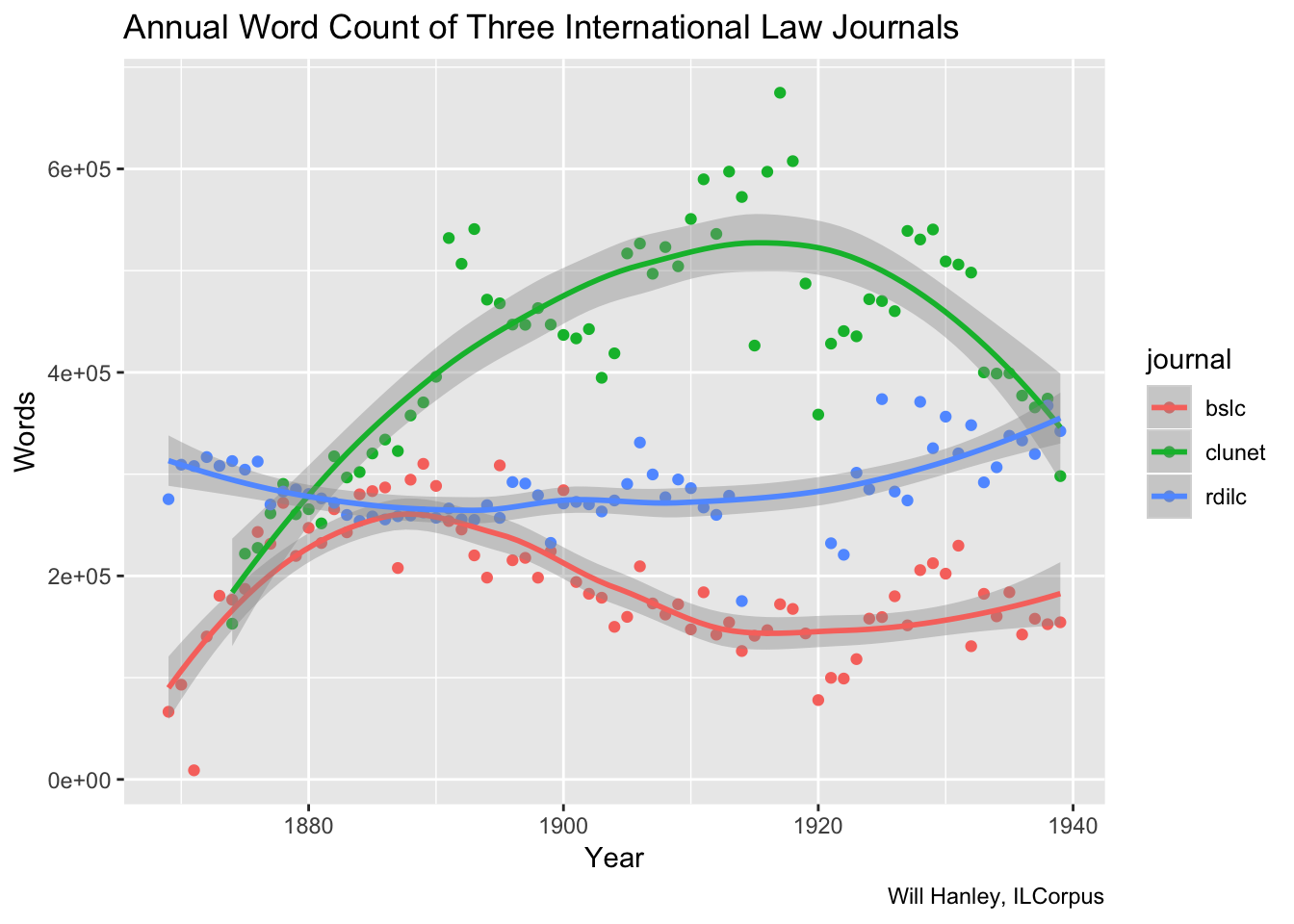
Individual points represent the total words of each year, while the smoothing line indicates trajectory.

Underlying code

These code blocks repeat the same steps for each of three journals. It might be good to figure out how to do all three in one step.

First, load text of all files

library(xml2)

bslc_files <- dir("~/GitHub/ilcorpus/journals/bslc/bslc-issues", full.names = TRUE)
bslc_text <- c()
for (f in bslc_files) {
  bslc_text <- c(bslc_text, gsub("\\s+", " ", paste(xml_text(xml_find_all(read_xml(f), "//text()")), collapse=" ")))
}

clunet_files <- dir("~/GitHub/ilcorpus/journals/clunet/clunet-issues", full.names = TRUE)
clunet_text <- c()
for (f in clunet_files) {
  clunet_text <- c(clunet_text, gsub("\\s+", " ", paste(xml_text(xml_find_all(read_xml(f), "//text()")), collapse=" ")))
}

rdilc_files <- dir("~/GitHub/ilcorpus/journals/rdilc/rdilc-issues", full.names = TRUE)
rdilc_text <- c()
for (f in rdilc_files) {
  rdilc_text <- c(rdilc_text, gsub("\\s+", " ", paste(xml_text(xml_find_all(read_xml(f), "//text()")), collapse=" ")))
}

Tokenize the words, then count them:

library(tokenizers)

clunet_words <- tokenize_words(clunet_text)
sapply(clunet_words, length)
bslc_words <- tokenize_words(bslc_text)
sapply(bslc_words, length)
rdilc_words <- tokenize_words(rdilc_text)
sapply(rdilc_words, length)

I prepared separate metadata summaries about each journal, drawing year and date from the TEI header of each file. These summaries will probably be useful in future steps. For now, get and use date metadata about every issue:

library(tidyverse)

bslc_metadata <- read_csv("~/GitHub/ilcorpus/journals/bslc/bslc-summary.csv")
clunet_metadata <- read_csv("~/GitHub/ilcorpus/journals/clunet/clunet-summary.csv")
rdilc_metadata <- read_csv("~/GitHub/ilcorpus/journals/rdilc/rdilc-summary.csv")

Now, produce a tibble for each journal, with each issue (there was more than one per year) its own observation. This tibble lists the issue, word count, and abbreviated title of the journal.

bslc_word_count <- tibble(year = bslc_metadata$year, words = sapply(bslc_words, length), journal = "bslc")
clunet_word_count <- tibble(year = clunet_metadata$year, words = sapply(clunet_words, length), journal = "clunet")
rdilc_word_count <- tibble(year = rdilc_metadata$year, words = sapply(rdilc_words, length), journal = "clunet")

Now cluster word counts by year:

clunet_word_count_year <- clunet_word_count %>% 
  group_by(year) %>% 
  summarise(words = sum(words), journal = "clunet")
bslc_word_count_year <- bslc_word_count %>% 
  group_by(year) %>% 
  summarise(words = sum(words), journal = "bslc")
rdilc_word_count_year <- rdilc_word_count %>% 
  group_by(year) %>% 
  summarise(words = sum(words), journal = "rdilc")

Put all three journals in a single tibble:

journals_count <- full_join(clunet_word_count_year, bslc_word_count_year)
journals_count <- full_join(journals_count, rdilc_word_count_year)

Plot the results as points and smoothing line

p <- ggplot(data = journals_count, mapping = aes(x = year, y = words, color = journal))
p + geom_point() + geom_smooth()

Plot the results as a streamgraph:

library(streamgraph)
streamgraph(journals_count, key="journal", value="words", date="year", offset="zero")

International Law Corpus

Visualizations of international law periodical content, 1869-1939.

Journal word counts over time

Underlying code